
How to Read and Analyze ELISA Data
Enzyme-linked immunosorbent assay (ELISA) data analysis involves converting absorbance or optical density (O.D.) measurements into target analyte concentrations using a standard curve. Accurate analysis requires appropriate curve fitting, evaluation of replicate variability, application of dilution factors, and verification that samples fall within the assay's validated range. This ELISA data analysis guide explains how to analyze ELISA results, generate and evaluate standard curves, calculate sample concentrations, assess replicate precision, and interpret ELISA data with confidence.
Steps for Analyzing ELISA Results
Analyzing ELISA results typically involves the following steps:
- Average replicate optical density (O.D.) values for standards, controls, and samples.
- Subtract the blank or zero standard O.D. value, if specified by the assay protocol.
- Generate a standard curve using the assay standards.
- Select and apply the appropriate curve-fitting model.
- Verify standard curve performance.
- Calculate unknown sample concentrations by interpolation from the standard curve.
- Apply any sample dilution factors to determine the final concentration.
- Evaluate replicate precision using the coefficient of variation (CV).
- Confirm that sample concentrations fall within the validated assay range and that sample O.D. values are within the limits of the standard curve.
Preparing ELISA Data for Standard Curve Analysis
Before generating a standard curve, calculate the mean optical density (O.D.) value for each standard, control, and sample from the replicate measurements. If specified in the assay protocol, subtract the average blank or zero standard O.D. value from each measurement to correct for background signal. The resulting values can then be used for standard curve generation and determination of unknown sample concentrations.
Creating an ELISA Standard Curve
Generate a standard curve by plotting the mean absorbance or optical density (O.D) values (y-axis) against the known standard concentrations (x-axis) and fitting the data using the curve-fitting method specified in the assay protocol. Standard curves are used to interpolate the concentrations of unknown samples from their measured absorbance values.
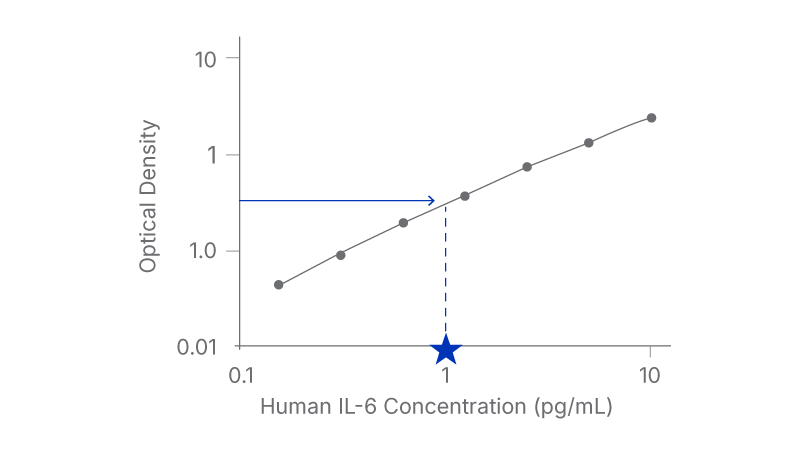
A representative standard curve is shown in the figure below from Human IL-6 HS Quantikine ELISA (Cat# HS600C).
| (pg/mL) | O.D. | Average | Corrected |
|---|---|---|---|
| 0 | 0.051 | 0.059 | - |
| 0.067 | |||
| 0.156 | 0.101 | 0.103 | 0.044 |
| 0.105 | |||
| 0.313 | 0.148 | 0.149 | 0.09 |
| 0.149 | |||
| 0.625 | 0.246 | 0.251 | 0.192 |
| 0.255 | |||
| 1.25 | 0.431 | 0.432 | 0.373 |
| 0.433 | |||
| 2.5 | 0.798 | 0.804 | 0.745 |
| 0.809 | |||
| 5 | 1.407 | 1.418 | 1.359 |
| 1.429 | |||
| 10 | 2.485 | 2.498 | 2.439 |
| 2.51 |
Choosing a Curve-Fitting Method
Use the curve-fitting method recommended in the assay insert whenever possible. If the recommended curve-fitting method is unavailable, evaluate alternative models such as linear, semi-log, log/log, 4-parameter logistic (4PL), or 5-parameter logistic (5PL) regression to determine which model provides the best fit for the standard curve data.
If curve-fitting software is unavailable, ELISA data may be linearized by plotting the log of the protein concentrations versus the log of the O.D. values and performing linear regression analysis. While this approach can provide an adequate estimate of sample concentrations, it is generally less precise than software-based curve-fitting methods.
Verifying Standard Curve Performance
A common way to assess standard curve performance is to back-calculate the standards. After generating the standard curve, treat the standards as unknowns and calculate their concentrations from the fitted curve. The calculated concentrations should closely match the expected values, generally within +/- 10%. When comparing different curve-fitting methods, select the model that provides the most accurate back-calculated values and the best overall fit to the standard curve.
Calculating Target Protein Concentration from an ELISA Standard Curve
To determine the concentration of each sample, use its absorbance value to interpolate the corresponding concentration from the standard curve. When interpreting a plotted standard curve manually, identify the sample absorbance on the y-axis, extend a horizontal line to the curve, then project vertically to the x-axis to determine the corresponding concentration.
Applying Sample Dilution Factors
If samples have been diluted before analysis, multiply the concentration determined from the standard curve by the dilution factor to calculate the final sample concentration.
Running Samples in Duplicate or Triplicate
Always run ELISA samples in duplicate or triplicate. Replicate measurements provide a means of assessing assay precision and identifying potential sources of variability. Average the duplicate or triplicate readings for each standard, control, and sample and evaluate agreement between replicates using the coefficient of variation (CV). For many ELISA applications, the CV of duplicate measurements should be ≤ 20%.
Evaluating Replicate Precision Using the Coefficient of Variation
The coefficient of variation (CV) is a measure of assay precision that compares the standard deviation of replicate measurements to their mean value. It is typically expressed as a percentage and can be used to evaluate agreement between duplicate or triplicate wells. Lower CV values indicate better reproducibility, while higher CV values may suggest issues with pipetting, plate washing, reagent handling, or other sources of experimental variability.
CV (%) = standard deviation/mean x 100
Calculating CV is important because it can help identify inconsistencies in ELISA results. For many ELISA applications, the CV of duplicates should be ≤ 20%. Higher CV values indicate greater variability between replicate measurements and may suggest experimental error.
Confirming Results Fall Within the Assay Range
Unknown sample concentrations should fall within the validated quantifiable range of the assay. Samples with concentrations that exceed the highest standard should generally be diluted and reanalyzed so that the measured value falls within the quantifiable range of the assay. Concentrations below the lowest validated standard should not be reported as quantitative results and are typically reported as being below the assay’s lower limit of quantification.
Optical density (O.D.) is a measurement of the amount of light absorbed by the colored reaction product generated during an ELISA. In sandwich ELISA formats, higher concentrations of the target analyte typically produce higher O.D. values. O.D. values from the assay standards are used to generate a standard curve, sometimes referred to as a calibration curve, which is then used to determine the concentration of the target analyte in unknown samples.
An acceptable standard curve should accurately describe the relationship between optical density (O.D.) and analyte concentration across the validated assay range. One common way to assess curve performance is to back-calculate the concentrations of the standards using the fitted curve and compare them with their expected concentrations. The back-calculated values should closely agree with the expected values across the standard curve range. Systematic deviations, poor recovery of individual standards, or large differences between expected and calculated concentrations may indicate that the curve-fitting model is inappropriate or that assay performance should be further evaluated. Acceptance criteria vary by assay, but standard recoveries and curve accuracy should meet the performance specifications established during assay validation.
A 4-parameter logistic (4-PL) curve fit is commonly used for ELISA standard curve analysis because many ELISA assays produce sigmoidal dose-response relationships that are not accurately described by a simple linear regression model. By modeling the shape of the standard curve across the full dynamic range of the assay, 4-PL analysis provides more reliable interpolation of unknown sample concentrations.
When sample volumes permit, running samples in duplicate or triplicate helps assess assay precision and identify potential errors during assay execution. Replicate measurements increase confidence in reported concentrations and provide a means of evaluating assay variability, often through calculations such as the coefficient of variation (CV).
The coefficient of variation (CV) is a measure of assay precision that reflects the variability among replicate measurements. Lower CV values indicate better agreement between replicates and greater assay reproducibility. As a general guideline, the CV for duplicate wells is typically expected to be ≤ 20%, although acceptance criteria may vary depending on the assay, sample type, and experimental requirements. Higher CV values may indicate increased variability caused by factors such as pipetting errors, inconsistent washing, sample handling, or other assay-related variables.
ELISA sensitivity refers to the lowest analyte concentration that can be distinguished from background signal, while the assay range defines the concentrations that can be accurately and reproducibly quantified using the standard curve. Analyte concentrations below the validated assay range may still generate a detectable signal, but only values within the validated assay range should be considered suitable for quantitative reporting.
If a target protein cannot be detected or accurately quantified, its concentration may be below the assay's limit of detection or outside the assay's validated quantifiable range. Reviewing the expected sample values provided in the kit documentation and consulting published literature can help determine whether analyte concentrations are expected to fall within the assay's measurable range. Non-detectable results may also be caused by factors such as sample degradation, matrix effects, assay interference, or use of a sample type that has not been validated for the assay. Results below the validated standard curve range should not be reported as quantitative values, even if a detectable signal is observed.
Generally, no. ELISA results should be reported only within the validated standard curve range of the assay. Concentrations below the lowest standard or above the highest standard fall outside the range where assay accuracy, precision, and quantitation have been established. While some software may generate extrapolated concentration estimates, these values are typically considered less reliable and should be interpreted with caution.
Samples with concentrations above the highest standard fall outside the assay’s validated quantification range and should generally be diluted and reanalyzed so that the measured value falls within the assay's validated range. The concentration obtained from the standard curve can then be multiplied by the appropriate dilution factor to determine the concentration in the original sample.
When samples are diluted before analysis, the concentration determined from the standard curve reflects the diluted sample rather than the original specimen. To calculate the concentration in the original sample, the value obtained from the standard curve should be multiplied by the dilution factor used during sample preparation. For example, if a sample is diluted 1:10 and the measured concentration of the target analyte is 50 pg/mL, the concentration of the analyte in the original sample is 500 pg/mL.
Looking for additional guidance on ELISA assay setup, reagent handling, pipetting technique, plate washing, incubation conditions, and methods for reducing assay variability? Review our 10 Best Practices and Techniques Guide.
Literature
- Soluble B7-H1/PD-L1 Levels in Multiple Cancer Subtypes: High Sensitivity Measurement by Immunoassay
- Improved Sensitivity of Vitamin D BP ELISA Kits
- A New Immunoassay for Detecting Anti-Zika Virus IgG with Very Low Dengue Cross-Reactivity
- A Novel, Quantitative, Multi-analyte Immunoassay to Detect Biomarkers Involved in Lung Disease
- A Novel Quantitative Multianalyte Immunoassay to Detect Peripheral Blood Biomarkers Following Traumatic Brain Injury